FLASH Tutorial#

This example shows how to draw the sequence diagram of the 2D FLASH sequence, as show, in FLASH imaging. Rapid NMR imaging using low flip-angle pulses, Haase et al., Journal of Magnetic Resonance, 67(2), pp. 258-266, 1986.

Start by creating two matplotlib objects, a figure and a plot, then create an empty sequence diagram which will be drawn in the matplotlib plot. The second argument is a list of channels: horizontal time lines for the various sequence events. Channel names may contain math expression inside dollar characters: they will be interpreted according to LaTeX rules. Channel names are arbitrary, and carry no specific meaning.

import matplotlib.pyplot
import mrsd

figure, plot = matplotlib.pyplot.subplots(figsize=(4,4), tight_layout=True)
diagram = mrsd.Diagram(
    plot, ["RF", "$G_{slice}$", "$G_{phase}$", "$G_{readout}$", "Signal"])

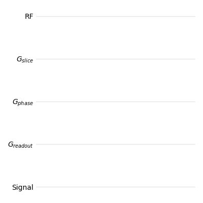
../_images/empty.png — Empty sequence diagram#

Slice-selective Pulse#

The 2D FLASH sequence starts with a slice-selective RF pulse, i.e. an RF pulse played concurrently with a gradient on the slice axis.

Within mrsd, everything that happens during a sequence (RF pulses, gradients, echoes, etc.) is called an event. Each event has a duration and a position in time, which can be specified by the begin, end or center of the event. This can be used to synchronize events: the RF pulse is centered on 0, and the slice-selection gradient is centered on the RF pulse.

We start by creating the RFPulse with a duration of 2 (time units are arbitrary), and an amplitude of 1 (amplitudes of events are normalized between -1 and 1). We then create the Gradient, with a flat-top centered on the pulse, and an amplitude of 0.5. Once created, those two objects are added (add()) to their respective channels.

pulse = mrsd.RFPulse(2, 1, center=0)
slice_selection = mrsd.Gradient(pulse.duration, 0.5, center=pulse.center)

diagram.add("RF", pulse)
diagram.add("$G_{slice}$", slice_selection)

It is also possible to directly add object to the diagram by calling the appropriate functions of the Diagram class: rf_pulse() and gradient().

pulse = diagram.rf_pulse("RF", 2, 1, center=0)
slice_selection = diagram.gradient(
    "$G_{slice}$", pulse.duration, 0.5, center=pulse.center)

Ramp times can be added to the gradients, using either the ramp parameter (symmetric ramp-up and ramp-down times), or both the ramp_up and ramp_down parameters (asymmetric gradients). These parameters can be used in both forms of gradient creation.

Since selective pulses are a common pattern, a convenience function (selective_pulse()) exists to create both objects:

pulse, slice_selection = diagram.selective_pulse(
    "RF", "$G_{slice}$", 2, gradient_amplitude=0.5, ramp=0.1, center=0)

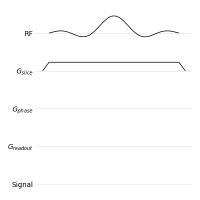
../_images/pulse.png — Slice-selective pulse#

The envelope of RF-pulses can be tuned using the envelope parameter: it defaults to sinc, but box or gaussian can also be used. You can also use the convenience functions sinc_pulse(), hard_pulse(), and gaussian_pulse() of the Diagram objects.

Readout#

The readout occurs at echo time, and comprises three events: the ADC being switched on and off, the Echo, and the readout gradient. As for the selective pulse, the objects can be created then added to the diagram. Note that the ADC object takes an extra parameter, ec: this is passed to matplotlib and can be used to change the aspect of the drawn object (color, line style, transparency, etc.).

TE = 4
d_readout = 2

adc = mrsd.ADC(d_readout, center=TE, ec="0.5")
echo = mrsd.Echo(d_readout, 1, center=adc.center)
readout = mrsd.Gradient(d_readout, 1, ramp=0.1, center=adc.center)

diagram.add("Signal", adc)
diagram.add("Signal", echo)
diagram.add("$G_{readout}$", readout)

The readout events can also be added using functions from the Diagram class: adc() and mrsd.Diagram.echo().

adc = diagram.adc("Signal", d_readout, center=TE, ec="0.5")
echo = diagram.echo("Signal", d_readout, 1, center=adc.center)
readout = diagram.gradient(
    "$G_{readout}$", d_readout, 1, ramp=0.1, center=adc.center)

As for the selective pulse, the readout is a common pattern for which a convenience function (readout()) can create all three events.

adc, echo, readout = diagram.readout(
    "Signal", "$G_{readout}$", d_readout, ramp=0.1, center=TE,
    adc_kwargs={"ec": "0.5"})

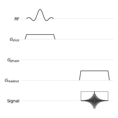
../_images/readout.png — Pulse and readout#

Encoding Gradients#

The phase-encoding gradient is displayed as overlayed gradient lobes to represent the different repetitions of the sequence: in mrsd, this is called a MultiGradient.

d_encoding = 1

phase_encoding = mrsd.MultiGradient(d_encoding, 1, 0.1, end=readout.begin)
diagram.add("$G_{phase}$", phase_encoding)

As for the other events, it can be directly added using a function from the Diagram class (multi_gradient()).

diagram.multi_gradient("$G_{phase}$", d_encoding, 1, 0.1, end=readout.begin)

The prephasing lobe of the readout gradient depends on the readout gradient itself: its area must be minus one-half that of the main readout lobe. Gradient events have an adapt() function which create a new gradient from an existing one and an area ratio.

readout_prephasing = readout.adapt(d_encoding, -0.5, 0.1, end=readout.begin)
diagram.add("$G_{readout}$", readout_prephasing)

Similarly, the slice-encoding gradient must be rewound.

diagram.add(
    "$G_{slice}$",
    slice_selection.adapt(d_encoding, -0.5, 0.1, end=readout.begin))

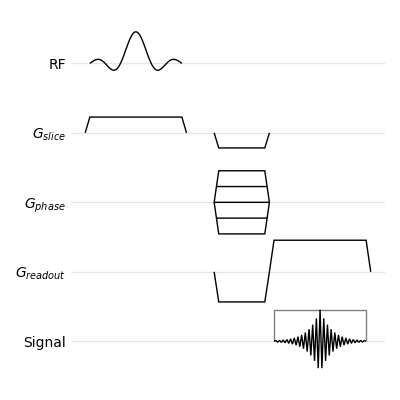
../_images/encoding.png — Pulse, readout, and encoding gradients#

Annotations and Copies#

The sequence diagram can be supplemented with annotations for a better understanding of the sequence. Time intervals (interval()) can show the TE and TR.

TR = 10

diagram.interval(0, TE, -1.5, "TE")
diagram.interval(0, TR, -2.5, "TR")

Channel specific annotations (e.g. flip angles and direction of phase encoding) are added using annotate().

diagram.annotate("RF", 0.2, 1, r"$\alpha$")
diagram.annotate("$G_{phase}$", phase_encoding.end, 0.5, r"$\uparrow$")

Finally, we show the beginning of the next repetition by creating copies of the RF pulse and the slice-selection gradient and moving them by the value of TR (move()).

diagram.add("RF", copy.copy(pulse).move(TR))
diagram.add("$G_{slice}$", copy.copy(slice_selection).move(TR))
diagram.annotate("RF", TR+0.2, 1, r"$\alpha$")

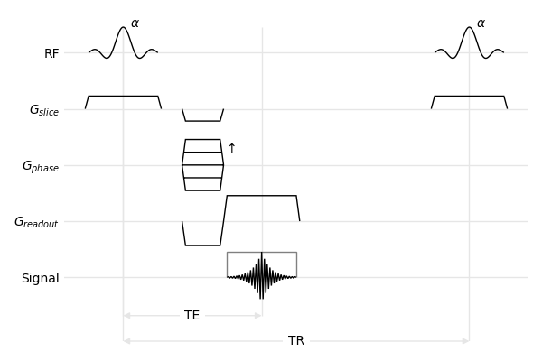
../_images/flash.png — Full diagram of the FLASH sequence#